Technical Notes
How OTOM models laser-assisted fibre placement and tape winding: the optical, thermal, crystallisation and residual-stress models, the numerics that keep them fast, and the link to the machine’s PLC.
Thank you for reading this post, don't forget to subscribe!OTOM is a physics-based optical-thermal simulation package for LATW, LATP and AFP. It is designed for in-line use, so computational efficiency matters as much as accuracy. Each model below is built to give an acceptable answer in the time the process allows.
The model chain
Kinematics
The tool is loaded from STL or STEP and the machine programme from G-code, XML or RAPID. Courses are projected onto the surface and the lay-up is built ply by ply, with the head and robot following the roller. Overlaps, tape deformation and roller deformation are taken into account.
Optics
The laser ray bundle is traced against the tool, the placed and incoming tape and the roller, including Fresnel absorption, reflections and a BRDF pattern that depends on fibre orientation. The output is the absorbed power on every surface along the path, and the shadowing that complex geometry causes.
Thermal
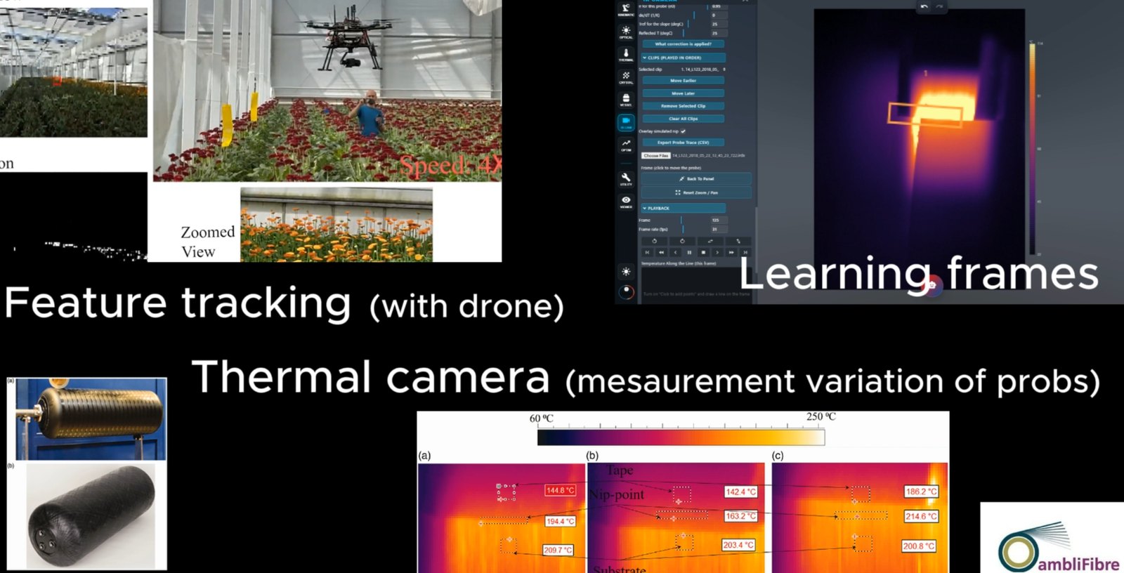
Three coupled models: the incoming tape (2D finite differences), the placed tape (3D finite elements) and the substrate (through-thickness columns, optionally cumulative over the whole lay-up). They give nip-point, interface and surface temperature histories that can be matched against thermal-camera measurements.
Crystallinity and residual stress
Crystallisation kinetics are integrated over the solved temperature history. A viscoelastic finite-element model then follows the stress in the laid tape through laying, cool-down and release from the tool.
Optimisation and control
Laser power and source position are adjusted per station to reach a target temperature, which gives proper bonding without degrading the material through overheating. Fast look-ahead methods make this usable in-line.
Numerics for speed
| Setting | Default | Alternatives and notes |
|---|---|---|
| Substrate equation solver | GPU (WebGPU) conjugate gradient | PCG on the CPU (most accurate) or Line SOR (the original). All three solve the same equations. |
| Laser ray trace | GPU | CPU. The first station is traced both ways; a difference over 2% switches back to the CPU automatically. |
| Pipelined laser trace | On | The next station’s trace is queued while the current substrate solves. The trace depends only on geometry, so results are identical. |
| Incoming tape solver | Line solver | An exact solve along the tape plus sweeps across the width. It agrees with the banded direct solve to about 1e-8 °C. |
| Adaptive sleep | Off | Skips settled nodes. It moves the substrate peak by only about 0.2 °C. |
Residual stress: method at a glance
8-node hexahedron with incompatible modes
A Wilson–Taylor element, equivalent to Abaqus C3D8I, with 2×2×2 Gauss integration. Plain hex8 elements lock in bending at the 3 mm by 0.1 mm aspect ratio of tape elements and under-predicted warpage about 7×.
Viscoelastic, transversely isotropic ply
A standard linear solid with temperature-dependent relaxation, in an incremental formulation that includes molten material and solidification. Defaults are literature values for AS4/PEEK, to be replaced with measured data.
Driven by the thermal FEM
Elements are born as the head lays them and contact follows the thermal model’s own classification. Cool-down and optional release from the tool follow.
Stress in the material frame
Fibre, transverse and through-thickness stresses in MPa, with a failure index and an HTML report. It runs on the GPU with a CPU reference solver.
In-line monitoring and PLC integration
Because the models run fast, OTOM can work alongside the machine instead of only before it. The original LATW implementation connects to Beckhoff TwinCAT over ADS to exchange process data with the PLC, and AFP Web reads thermal-camera recordings or live streams for comparison with the simulation.
- A fast algorithm for in-line monitoring
- A general mandrel model, including analytical cylinder and dome geometry
- Line and probe profiles, adaptive nip-point tracking and a report
Want the full technical detail?
We share method documents and validation results with customers and research partners.