Technical Feasibility
Before a project starts, we check that the physics, the numerics and the hardware can answer your question, whether it concerns fibre placement, fluid flow or particle and melt behaviour.
Thank you for reading this post, don't forget to subscribe!Every project brings new challenges. A short, structured feasibility check tells you early what can be predicted, how accurately and how fast, so the engineering budget goes where it pays off.
How a feasibility study runs
Evaluation (1–3 weeks)
We assess your case against the capabilities of OTOM AFP Web, OTOM CFD and OTOM SPH, and give you clear feedback on what can be modelled and with what confidence.
Quotation
If the evaluation is positive, we prepare a quotation that covers engineering hours, computing hardware and travel, including a one- to two-day visit to your production site for data acquisition.
Data acquisition and set-up
Geometry, machine programme, materials and process settings are collected and structured into model inputs.
Simulation, validation and report
Results are compared with measurements or manufactured parts and delivered as a recommendation with plots, animations and an HTML report.
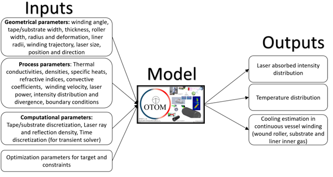
Data structure: inputs and outputs
- Geometrical: tool and part (STL/STEP), laser head, roller, obstacles
- Process: machine programme (G-code, XML, RAPID), speed, laser power, material properties
- Computational: grid and time step, solver choice, analysis range
- Kinematics: course mapping and ply-by-ply lay-up
- Optical: absorbed laser power on every surface
- Thermal: nip, interface and surface temperature histories
- Optimisation: laser power or source position per station
The numerical methods we bring
| Domain | Methods | Feasible questions |
|---|---|---|
| Composites (AFP, LATP, LATW) | GPU ray tracing with Fresnel absorption; 2D finite differences for the incoming tape; 3D finite elements for the placed tape; through-thickness substrate columns; crystallisation kinetics | Nip-point temperature, laser shadowing, bonding quality, crystallinity of PEEK, PEKK and PPS, and laser power optimisation |
| CFD | Incompressible Navier-Stokes by Chorin projection with a pressure Poisson solve; compressible Euler by finite volumes with the HLLC Riemann solver; Brinkman penalisation for walls; Smagorinsky LES; vorticity confinement | Drag and lift, separation and vortex shedding, shocks up to Mach 5, ventilation, two-fluid stratification |
| SPH | Weakly compressible SPH with Spiky kernels; SPS-LES turbulence; log-law wall model; streamlines and pathlines | Free surfaces, filling, mixing, hopper discharge, and high-viscosity melt flow around fibre bundles |
Real-time results through parallel GPU computing
All three engines run on WebGPU compute shaders, in the browser and on the user’s own graphics card. That is what makes interactive engineering possible without a workstation, a cluster or uploaded data.
Pipelined GPU thermal solver
A conjugate-gradient substrate solve on the GPU, with the next station’s laser trace queued while the current one solves. The first station is traced on GPU and CPU and compared; a difference over 2% falls back to the CPU.
Fused, stable kernels
The four HLLC face fluxes and the cell update run in one compute pass. A positivity guard keeps strong shocks free of NaNs, and grids reach 4096 cells across in 2D.
Sorting at scale
A parallel prefix sum over a linear grid finds particle neighbours, density splatting uses fixed-point atomics, and frustum culling with indirect dispatch keeps tens of thousands of particles at 60 FPS.
| AFP Web thermal run (Fraunhofer IGCV funnel, two plied paths) | Time |
|---|---|
| Original CPU solvers | 32 s |
| GPU substrate solver + GPU laser ray trace | 16.6 s |
| Hidden overheads removed, fewer GPU round trips | 7.5 s |
| Pipelined laser trace (current default) | 6.1 s, about 5.6× faster with identical temperatures |
Feasibility in practice
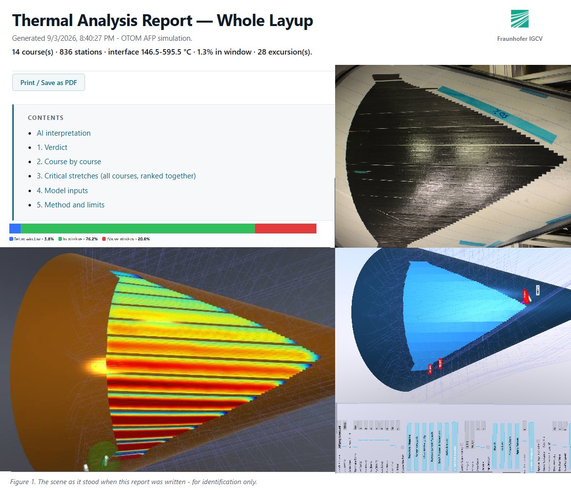
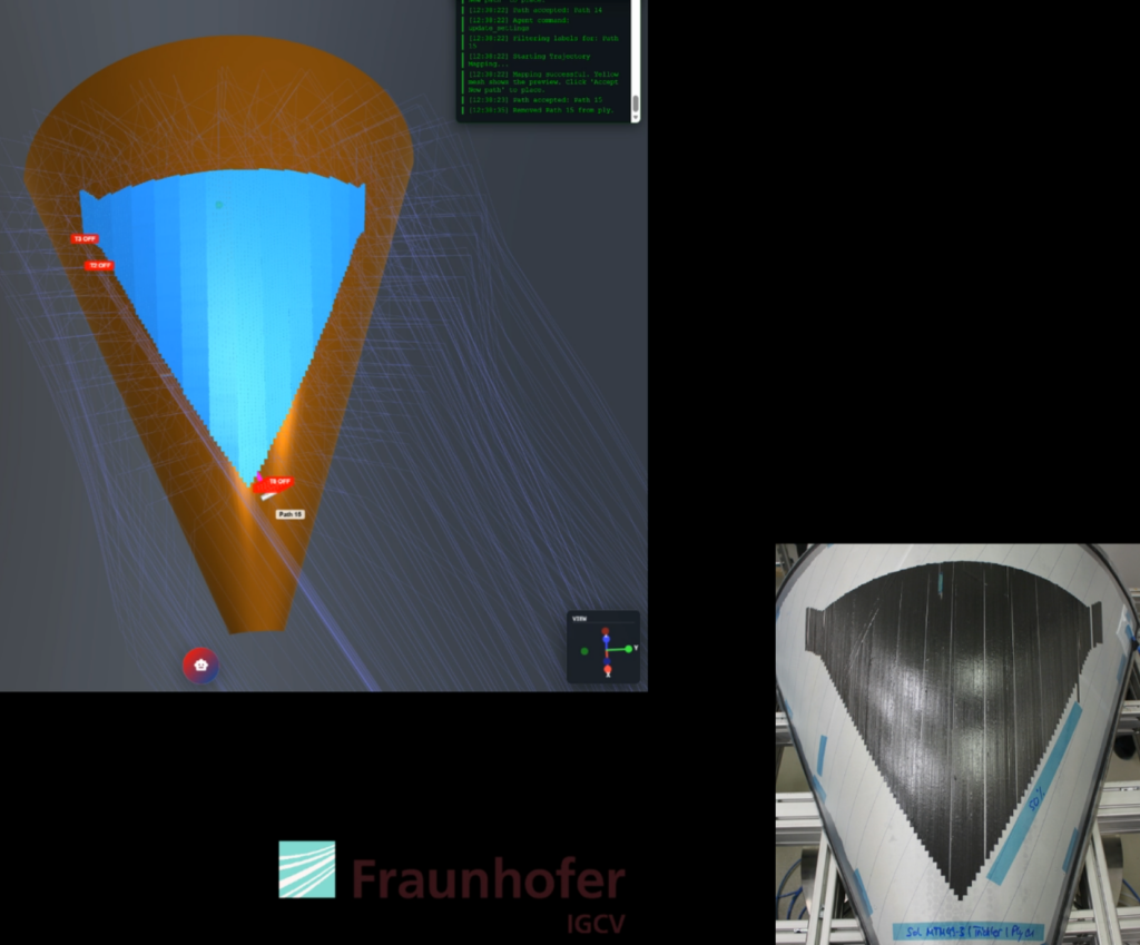
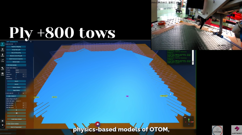
Two recent AFP Web cases compare the simulated lay-up with the part on the machine: a conical funnel made with Fraunhofer IGCV, and a flat panel of more than 800 tows placed on a LAYWAY AFP machine.
For flow, the same approach produced a CFD digital twin of greenhouse ventilation at Herenboeren Usseler Es in Enschede; see the case study.
Is your case feasible?
Send us a short description and a drawing. You will hear back within one to three weeks.