Residual Stress
Every placed course cools, crystallises and shrinks while it is held by the tool and by the plies beneath it. OTOM AFP Web follows that history and predicts the stress locked into the part, and the warpage when it comes off the tool.
Thank you for reading this post, don't forget to subscribe!Residual stresses in AFP parts are not a surprise. They come from the thermal history and from constrained layers that want to expand and shrink by different amounts. They lead to delamination, distortion and early failure, and they weaken interlaminar fracture toughness. The question is how big they are, and where.
Four sources of stress
- Thermal contraction: fibre and matrix expand very differently (about 0.2 against 28–75 µε/K for AS4/PEEK)
- Crystallisation shrinkage: the matrix shrinks as it crystallises
- Through-thickness gradients: a hot top and a cooler bottom bend each course
- Constraint: the tool and earlier plies stop the tape from moving freely
What is computed: the three phases
Each element is born, stress-free, as the head passes, and starts carrying stress where it solidifies. A later pass that re-melts it erases its stress.
The part cools to room temperature while still bonded to the rigid tool. Viscoelastic relaxation acts throughout.
The tool bond is removed and the held stress redistributes. The spring-back is the warpage, reported relative to the best-fit position, as a measured part would be judged.
Stresses are reported in each element’s material frame: σ11 along the fibre, σ22 transverse in-plane and σ33 through the thickness, plus the interlaminar shears, in MPa.
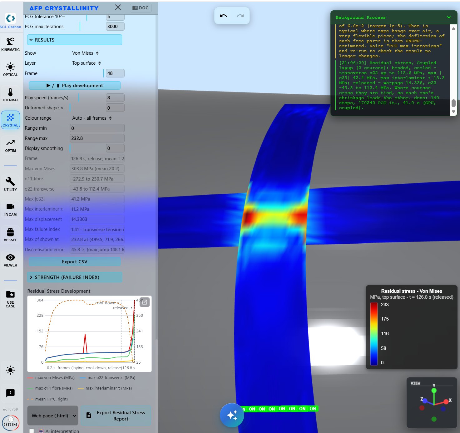
The model, driven by the real process
The residual-stress module ports our original MATLAB viscoelastic codes into AFP Web. Where the MATLAB model cooled a part uniformly, here every element follows the temperature history of the actual AFP process from the thermal finite-element model, and the crystallinity from the Crystal tab.
Hexahedron with incompatible modes
Tape elements are about 3 mm long and 0.1 mm thick. A plain 8-node brick locks in bending at that aspect ratio and under-predicted warpage about 7×. OTOM uses the Wilson–Taylor element with incompatible modes (equivalent to Abaqus C3D8I), which passes the patch test.
Viscoelastic, transversely isotropic
A standard linear solid in which the matrix-dominated moduli relax and the fibre modulus does not. The relaxation time follows WLF above Tg and an exponential law below it. Stress builds incrementally, so material that solidifies does so stress-free.
Thermal and crystallisation strains
The transverse expansion coefficient switches at Tg, and shrinkage scales with relative crystallinity from Nakamura or dual-Avrami kinetics, including melting. Temperature and crystallinity are interpolated to every Gauss point, which keeps the through-thickness gradient that bends a course.
Coupled courses with surface ties
All courses run in one model. Each is tied to the course beneath with a surface-to-surface penalty tie (like Abaqus *TIE), so crossing courses with non-matching meshes join without artificial stress peaks. Earlier courses are reheated, or re-melted, when a later one crosses them.
Solved on the GPU, checked on the CPU
Matrix-free CG on WebGPU
Element kernels and a node gather, with no float atomics, and reductions on the GPU. The same algorithm runs in double precision on the CPU as fallback and reference. GPU and CPU warpage agree: 1.254 against 1.253.
Column-block preconditioner
Thin plies couple top and bottom nodes far more strongly than in-plane. Inverting each through-thickness column block solves that exactly: convergence in 1,671 iterations, where Jacobi had not converged after 20,000.
Direct solve for release
A free, thin course is too ill-conditioned for CG. Release uses a banded Cholesky factorisation after reverse Cuthill–McKee reordering. It takes under a second on the funnel lay-up.
Verified against analytical solutions
| Test | Expected | OTOM |
|---|---|---|
| Strip bonded at the bottom, cooled uniformly | 14.286 MPa | 14.286 MPa |
| Same strip released | stress-free | 0.000 MPa |
| Relaxation at time step = τ | viscous part halves each step | halves, then settles |
| Free strip, through-thickness gradient (corner deflection) | 4.83 | 4.72 (−2.4%) |
| Tied two-layer strip (Timoshenko bimetal) | 3.63 | 3.54 (−2.4%) |
| Same, with non-matching meshes | 3.63 | 3.52 (−3%) |
What you get
Results
- Contours of von Mises, σ11, σ22, σ33, τ12, τ23, τ13 and displacement
- Development of peak stresses over the lay-up
- Warpage after release from the tool
- A per-course table and an HTML report, with optional AI interpretation
Judgement
- Max-stress failure index, with the governing mode and its location
- Zienkiewicz–Zhu error estimate: below 10% means well resolved
- The CG residual reached, with a warning if it is too high
- Mesh-convergence check at 1× and 2× refinement
Predict distortion before the first part
Run the residual-stress analysis on your lay-up, or let us do it with your tape data.