CFD

https://otomcomposite.eu/CFD/

OTOM CFD executes high-performance fluid simulations directly inside modern web browsers using WebGPU, pairing an incompressible Navier–Stokes solver with a compressible Euler (HLLC) engine for shocks and transonic flow. Both 2D and 3D domains are supported, with 3D adding volumetric raymarching, physically-based rendering and isosurface extraction.

Fundamentals of the Model

OTOM CFD solves the actual equations of fluid motion on a grid every frame, rather than replaying precomputed data. Two solvers cover the two flow regimes.

Incompressible flow — pressure projection

For low-speed flow, the incompressible Navier–Stokes equations are solved:

$partial_t u + (ucdotnabla)u = -tfrac{1}{rho}nabla p + nunabla^2 u,quad nablacdot u = 0$

Each step splits into an advection–diffusion pass (velocity carried semi-Lagrangian along its own flow, viscosity diffused) followed by a projection: a pressure Poisson equation is solved with Jacobi iteration and used to remove any remaining divergence, so the field stays incompressible:

$nabla^2 p = tfrac{rho}{Delta t}nablacdot u^{*},quad u^{n+1}=u^{*}-tfrac{Delta t}{rho}nabla p$

Turbulence: Smagorinsky LES

The grid can’t resolve every eddy, so unresolved (sub-grid) motion is modelled as an added eddy viscosity proportional to the local strain rate:

$nu_t = (C_s Delta)^2 |S|,quad |S| = sqrt{2 S_{ij}S_{ij}}$

Vorticity confinement then adds a small compensating force to counter the extra numerical dissipation this smoothing would otherwise introduce, keeping resolved vortices from washing out.

Geometry without meshing: BDIM

Rather than generating a body-fitted mesh for every obstacle, the Boundary Data Immersion Method blends the fluid velocity with a prescribed solid velocity using a smoothed function of the signed distance $d$ to the nearest surface:

$u = mu(d), u_{fluid} + (1-mu(d)), u_{solid}$

Because this is analytical rather than a conformal mesh, obstacles can move, spin or deform every frame at essentially no extra cost — there’s nothing to re-mesh.

Shocks & transonic flow: compressible Euler / HLLC

When flow speeds approach or exceed the speed of sound, incompressible assumptions break down, so OTOM CFD switches to a finite-volume solver for the conservation laws of mass, momentum and energy:

$partial_t U + nablacdot F(U) = 0$

Fluxes at each cell face are resolved with an HLLC approximate Riemann solver, and positivity guards prevent density or pressure from going negative across strong shocks. All of this — both engines, on a staggered Cartesian grid — runs as fused WebGPU compute kernels, one pass per physics step.

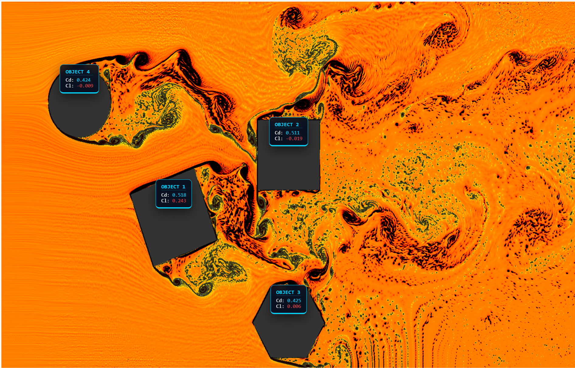
☆ Smagorinsky Large Eddy Simulation turbulence with vorticity confinement
☆ Boundary Data Immersion Method (BDIM) for arbitrary moving geometry, no meshing required
☆ Multi-phase flow with advected density/viscosity fields and Boussinesq gravity
☆ Spinning obstacles (Sphere, Box, Cylinder, Wing) or uploaded STL meshes, up to 4 secondary obstacles
☆ Surface-integrated drag, lift and torque, with Reynolds number computed live

Visualization & Analytics

Nine colormaps (Seismic, Jet, Hot, Viridis and more) with independent min/max windowing, log scaling and contour overlays let you inspect vorticity, velocity, pressure, phase fraction or Schlieren (pressure-gradient) fields. A Lagrangian particle system traces massless tracers through the flow, and the Ground Truth panel cross-checks measured drag/lift coefficients against empirical correlations for canonical shapes — cylinders, spheres, airfoils, prisms — with regime guidance.

Temperature, Buoyancy & Ventilation

An optional Boussinesq natural-convection module advects a temperature field with fixed-temperature or heat-flux zone sources, coupling buoyancy forces with pressure projection to drive self-consistent, wind-driven flow. Up to 4 ventilation fans (duct-style Box or rotor-style Disk models) can be placed to study inlet/outlet air movement — the kind of setup used to study natural and forced ventilation in an enclosed structure.

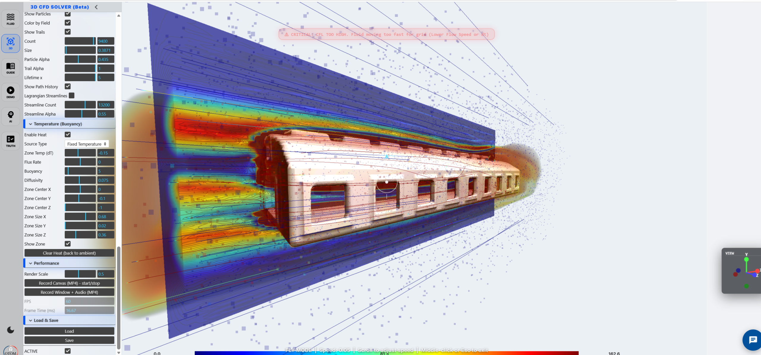
Example: temperature-driven ventilation airflow through a greenhouse, solved with the Boussinesq buoyancy module and SI Units Mode so results read out in real-world m/s and °C rather than lattice units.

Calibration & AI Assistance

SI Units Mode converts lattice quantities to real-world units from two calibration inputs (domain width and real-world time step), auto-validating CFL number and Reynolds regime and auto-correcting viscosity for Air, Water, Oil or Glycerin. An integrated CFDChatbot translates natural-language requests into parameter and geometry changes, and a local, browser-side assistant can explain the current scene (drag, lift, Reynolds, regime) without inventing values. An experimental neural-network surrogate mode can also be trained (2D U-Net or 3D CNN) to approximate results at much lower compute cost.

Full technical documentation: https://otomcomposite.eu/CFD/documentation.html

try it here: